Build your own single hippocampal cell model using HBP data
This Use Case allows a user to configure the BluePyOpt to run an optimization choosing from HBP data for morphology, channel kinetics, features, and parameters. The current version allows to select among self-consistent configuration files from previous optimizations.
By selecting this Use Case, three Jupyter Notebooks are cloned in a private existing/new Collab. The cloned Notebooks are:
BuildOwn Single HippoCell - Config
This allows the user to:
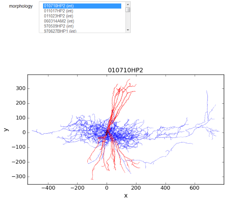
1 Choose and visualize an existing morphology from HBP data (the name and type of morphology are listed):
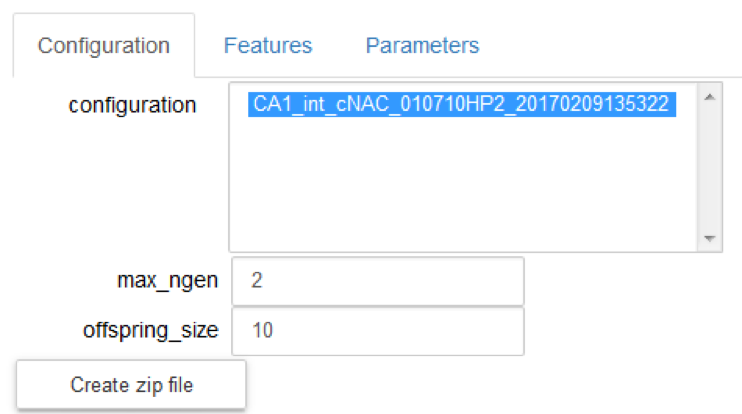
2 Choose a self-consistent set of configuration files (the four JSON files) for the chosen morphology; the list includes those available for the selected morphology:
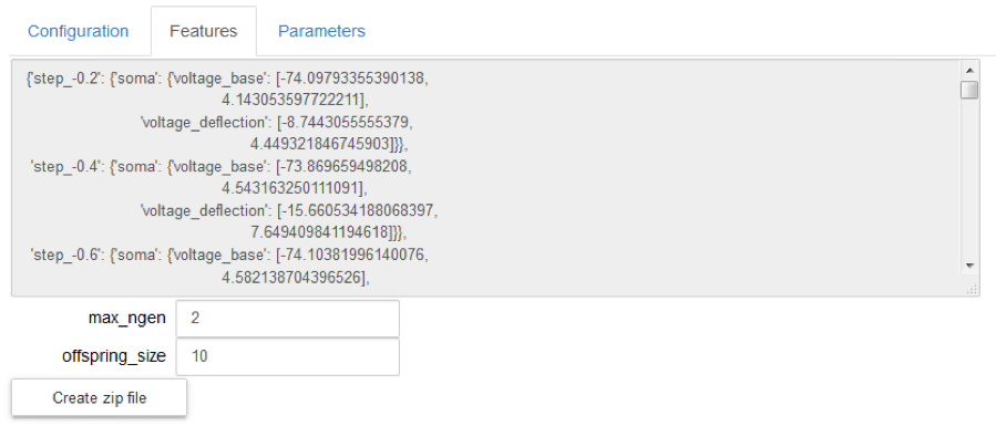
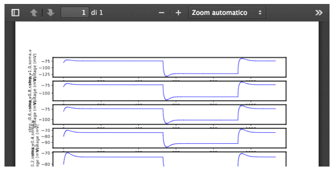
3 visualize the electrophysiological features that will be used as reference by the optimization process (“Features” tab); they cannot be changed; they are taken from the ‘features.json’ file.
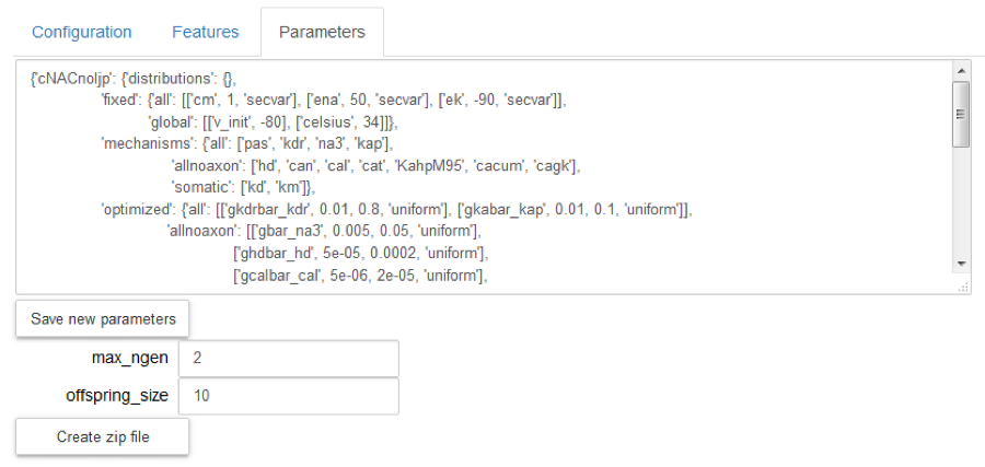
4 Visualize and change the parameters of an existing optimization (“Parameters” tab). The user can change the values and save them by using the “Save new parameters” button:
5 Configure the BluePyOpt optimization algorithm, by defining the offspring size and the max number of generations; they are set by default to 10 and 2 respectively.
6 Generate the zip file needed to run the new optimization by “Create zip file”.
7 Log in to NSG (Neuroscience Gateway) by inserting his/her username and password and clicking on the “Login NSG” button:
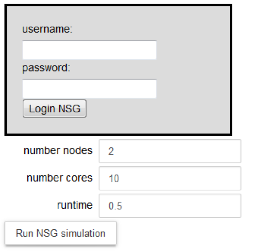
8 Configure the parameters of the optimization job: number of nodes, number of cores and runtime. They are set by default to 2, 10 and 0.5 respectively. The maximum number of nodes available per job is 72. If you would require more than 72 nodes please contact us at nsghelp@sdsc.edu. The maximum number of cores required per node is 24.
9 run the optimization by clicking on the “Run NSG simulation”.
10 the job has been submitted when you see:
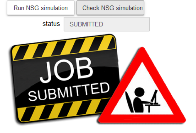
You may check the job status by clicking on the “Check NSG simulation”. The status may be: QUEUE, COMMANDRENDERING, INPUTSTAGING, SUBMITTED, LOAD_RESULTS or COMPLETED
Once the job is COMPLETED, results are saved in the Collab storage, under the BluePyOptAll/resultsNSG/username/foldername (foldername is the name of the configuration set, where date and time are updated with the current date and time).
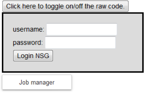
11 If you are interested in looking at the code, click on “Click here to toggle on/off the source code” button:

BuildOwn Single HippoCell - NSG Job Manager
This Jupyter Notebook allows the user to:
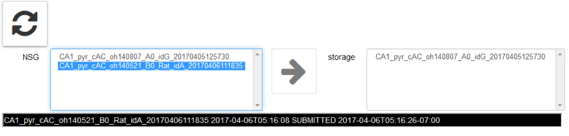
Log in to the Neuroscience Gateway (NSG) and load the Job Manager by clicking on “Job manager”:
eopy completed jobs from NSG to the Collab storage by clicking on the arrow icon →
Refresh jobs on the NSG by clicking on
 :
:
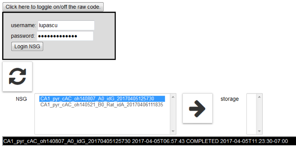
A job can be stored only if completed:
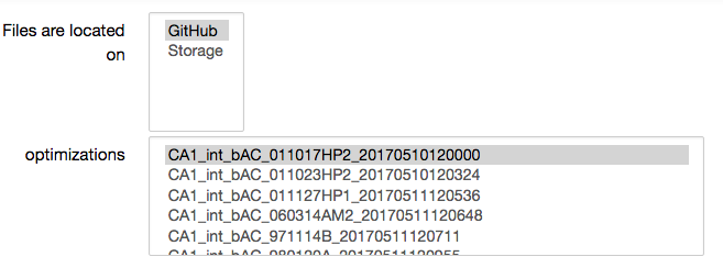
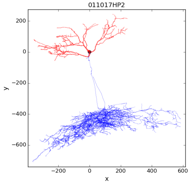
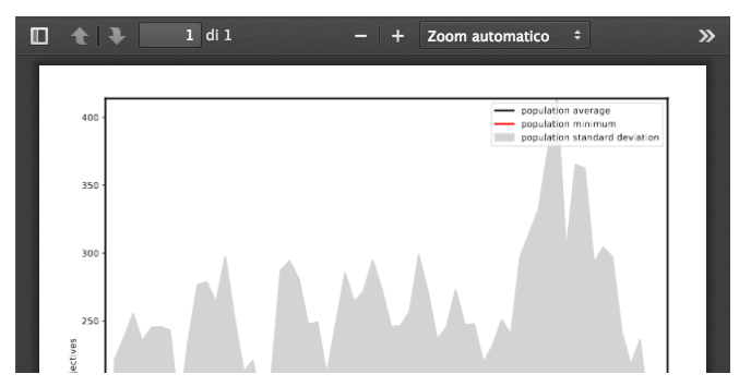
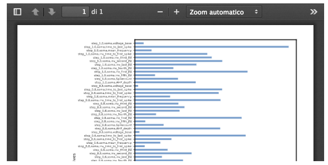
BuildOwn Single HippoCell - Analysis
This Jupyter Notebook allows the user to:
Choose either a previous optimization from the HBP GitHub repository; or choose the result of your own optimization from the Collab storage, and then run an analysis by clicking on “View analysis”
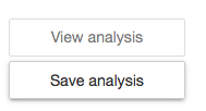
Save the analysis in the storage by clicking on “Save analysis”. The analyses are saved under the BluePyOptAnalysis/username/foldername (foldername is the name of the optimization)
If you are interested in looking at the code, click on “Click here to toggle on/off the source code” button:
